Riemann Sum Assignment

Approximating Area Under a Curve

The focus of this assignment will be defining and calculating the area under a curve. The following slides contain an introduction to the concept of Riemann sums, which provide a way of approximating this area:

Area Under a Curve Slides

We have seen that as the width of the rectangles in a Riemann sum gets smaller the approximation to the area under the curve improves. In some cases, we’ve been able to use this fact to compute the exact value of the area under the curve. In many cases, though, the sum is too complicated to be computed by hand.

This is where computers can be of help. Calculating a Riemann sum requires adding up many small areas to get an approximation of the total area under the curve. Computers are good at this kind of repetitive task: while there are many steps, the calculation involved in each step is simple. Remember how to tell a program to do the same thing over and over using for and while-loops? Now, you will apply this knowledge to create a Java class which evaluates a given Riemann sum.

The individual rectangles’ areas can be added up using a for-loop. The more iterations (steps) of the loop, the better the approximation.

Optional Exercise

The syntax of for-loops in Java can be hard to remember.

• Use a for-loop to print the first 100 positive integers.
• Use a for-loop to add up the first 100 positive integers.
• Use a for-loop and an array to find the mean of the following ten numbers: 28.2, 14.7, 10.3, -2.0, 55.8, 10.3, 0.2, 1.0, 0.0, 25.1

Classes and Methods

You will create several classes for this assignment: a base class called AbstractRiemann and then child classes for each of the Riemann sum rules.

The AbstractRiemann Class

The first class which you will create for this assignment, AbstractRiemann, will contain the majority of your code for calculating Riemann sums. Start by opening up the documentation for AbstractRiemann. The linked page, known as a JavaDoc, has information about each of the methods of the AbstractRiemann class. This includes the methods’ parameters (inputs) and their return values (outputs). Your job will be to create a class which conforms to the given JavaDoc—the AbstractRiemann class which you create should contain each of the listed methods, and each method should behave as described in the AbstractRiemann JavaDoc, taking in the same parameters and outputting the same type of return value.

Note

Java programmers frequently use JavaDocs to document their code so that other people can understand what it does. JavaDocs are created by writing comments in your source code using a specific format; you can find a good introduction to documenting your code in this way at https://alvinalexander.com/java/edu/pj/pj010014.

Abstract Classes and Methods

The AbstractRiemann class, as shown in the AbstractRiemann JavaDoc , contains a keyword which you most likely have not yet encountered: abstract. This keyword will allow you to use to use object-oriented programming (OOP) to organize your code in a more logical way.

You have learned that there are several different rules which can be used to calculate Riemann sums, such as the left hand rule, right hand rule, and trapezoid rule. Thinking of a Riemann sum as the sum of many small slices of the total area, these rules correspond to different ways of defining the slices. However, the overall method for calculating a Riemann sum remains the same; given the endpoints of the interval on which to calculate the sum and the number of slices, the calculation can always be divided into the following steps:

1. Calculate \(\Delta x\) (the width of each subinterval) from the endpoints of the interval and the number of slices.
2. Determine the endpoints of each subinterval.
3. Calculate the area of each slice.
4. Add up the areas to find the total area.

Notice that only the third step—calculating the area of each slice—depends upon the specific rule being used; the others are the same regardless of the rule.

Here, three different rules are being used to calculate the same Riemann sum. While the slices’ shapes are different, they exist over the same subintervals in each diagram.

Fortunately, Java provides a convenient means of structuring classes which are mostly the same but differ with respect to certain functions: inheritance. You will discuss this concept in class, and the following pages are recommended for reference:

• Oracle - Inheritance Tutorial
• Oracle - Abstract Tutorial

As shown in the AbstractRiemann JavaDoc, the AbstractRiemann class which you will create will be an abstract class. As such, you will never directly construct a new AbstractRiemann(); instead, you will create child classes (also known as extended classes or subclasses) of AbstractRiemann for each Riemann sum rule. In this way, you will end up with a structure where RightHandPlot and LeftHandPlot, both child classes of AbstractRiemann, share most methods, differing only in their implementations of getSubintervalArea() and drawSlice(), since these are the only methods whose functionality should depend on the rule.

See the Riemann Sum JavaDoc to see how the abstract class is different from the child classes.

For example, this is what a fictional rule called OvalPlot could look like:

public class OvalPlot extends AbstractRiemann {
    @Override
    public double getSubintervalArea(Polynomial poly, double leftBorder, double rightBorder) {
        // return the area of an ellipse whose width is (rightBorder - leftBorder)
        // and whose height is the polynomial evaluated at leftBorder
    }

    @Override
    public void drawSlice(PlotFrame pframe, Polynomial poly, double leftBorder, double rightBorder) {
        // draw an ellipse whose width is (rightBorder - leftBorder)
        // and whose height is the polynomial evaluated at leftBorder
    }
}

As shown in OvalPlot, you do not have to reimplement all of the methods in AbstractRiemann. Only the abstract methods should be written out in the subclasses.

Assignment

Remember to document as you go. Each method you write should have a documentation comment (ideally in the JavaDoc format) before it:

/**
 * [DESCRIPTION OF WHAT THE METHOD DOES]
 *
 * @param left [DESCRIPTION OF THE 'left' PARAMETER]
 * @param right [DESCRIPTION OF THE 'right' PARAMETER]
 * @param subintervals [DESCRIPION OF THE 'subintervals' PARAMETER]
 * @return [DESCRIPTION OF WHAT THE METHOD RETURNS]
 */
public double calculateDeltaX(double left, double right, int subintervals) {
    // the actual method
}

Base Assignment

You will write a total of eight Java classes for the base assignment. Together, they will demonstrate three Riemann variations: Righthand Rule, Lefthand Rule, and Trapezoid Rule.

See the Riemann Sum JavaDoc for an overview of all the classes in this project.

1. Create a Package Namespace

A good way to organize all the projects you will do this year is by creating a separate package namespace for each.

Exercise

Summary: Create a package namespace to hold your project.

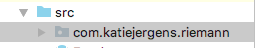
1. In src, right-click to get the option menu.
2. Select New…Package
3. Name it com.[yourname].riemann (E.g. if your name is Kim Cheng, name it com.kimcheng.riemann)

When your folder looks like the following you are done with this exercise:

2. AbstractRiemann Class

Exercise

Summary: Create an abstract class that has logic common to all Riemann rules.

1. In com.[yourname].riemann create the AbstractRiemann abstract class based on the AbstractRiemann JavaDoc .
2. Create all the attributes: poly, plotFrame, xLower, xUpper, and subintervals.
3. Create a constructor.
4. Write the non-abstract methods: calculateDeltaX(), getIntervalArea(), drawRiemannSlices(), plotPolynomial(), plotAccFnc(), and configPlotFrame().
5. For the accumulation function, plotAccFnc(), note that it graphs how the area grows with increasing \(x\). See Area Under a Curve Slides for a deeper explanation of the accumulation function.
6. Add stubs for the the abstract methods getSubintervalArea() and drawSlice(). Make sure to mark them as abstract and end the line with a semicolon instead of implementing the method.

3. RightHandPlot, LeftHandPlot and TrapezoidPlot

Exercise

Summary: Create object classes for various Riemann rules.

1. In your riemann package, create three child classes: RightHandPlot, LeftHandPlot, and TrapezoidPlot, each extending AbstractRiemann.
2. Each rule should implement the abstract methods getSubintervalArea() and drawSlice(). Do not include implementations of any other methods from AbstractRiemann; they will be automatically inherited.
3. For drawSlice(), make sure the plots correspond to the specific rules. Note: You don’t need to fill in the trapezoids for TrapezoidPlot.

4. Test Classes

Exercise

Summary: Test the Riemann getSubintervalArea() methods.

1. In the test folder, create a class called RightHandPlotTest and add a test method called slice that does the following:

• Creates a Polynomial (first import org.dalton.polyfun.Polynomial). E.g.,

Polynomial poly = new Polynomial(new double[]{3, 4, 2});

• Creates a RightHandPlot object. E.g.,

RightHandPlot rightHandPlot = new RightHandPlot(poly, new PlotFrame("x", "y", "Right Hand Rule"), 0, 2, 10);

• Asserts that the object’s getSubintervalArea() returns the correct area of the rectangle under the given Polynomial between two \(x\) values. You can check what the Riemann sum should be using a Riemann Sum Calculator.

You may add more test methods as you see fit. When you are certain RightHandPlot’s getSubintervalArea() method works, test the other rules:

1. In the test folder, create a class called LeftHandPlotTest that contains at least one method to test LeftHandPlot’s getSubintervalArea().
2. In the test folder, create a class called TrapezoidPlotTest that contains at least one method to test TrapezoidPlot’s getSubintervalArea().

When all the test methods pass you are done with this exercise.

5. RiemannApp

Exercise

Summary: Plot the Riemann rules.

1. Back in the riemann package, create RiemannApp, which will have a main method and be responsible for plotting example Polynomials, Riemann rectangles, and printing the estimated area.
2. Create an example Polynomial to find the area under. E.g., \(3x^2-6x+3\). See the Polynomial JavaDoc for how to construct a Polynomial.
3. For each plot object use drawRiemannSlices() to plot rectangles under the example Polynomial onto the cooresponding PlotFrame. E.g.,

rightHandPlot.drawRiemannSums();

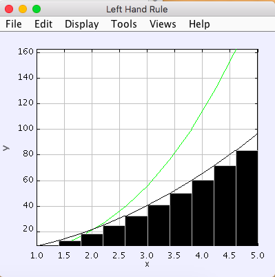
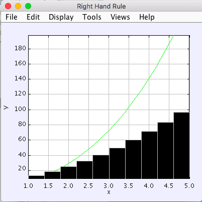
1. Also on each PlotFrame, call plotPolynomial() to plot the example Polynomial so you can see the line in relation to the rectangles.
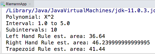
2. Plot the accumulation function using plotAccFnc().
3. Finally, for each rule, print the estimated area under the curve.

When your RiemannApp (1) prints estimated areas of a polynomial for each of the rules, (2) plots each rule and (3) plots each accumulation function you are done with this exercise.

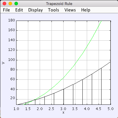
Example output:

1. Estimated areas of a polynomial:

2. Plots for each rule. The accumulation function is shown in green:

6. Analysis

Use your program to answer the following question: which of the three rules is the most accurate? This should compare the results of the Riemann sums with the actual area under the curve (use this Integral Calculator to get the actual value).

Warning

Remember to account for the following edge cases:

• The value of the polynomial for a given \(x\) is negative.
• The left endpoint is greater than the right endpoint.

Extension

The three Riemann sum rules which you have seen so far (the right hand rule, left hand rule, and trapezoid rule) tend to yield good approximations of the area under a curve provided that \(\Delta x\) is small enough. However, they are not the only rules.

For your extension, research different Riemann sum rules and write classes for them in the same style as the base assignment. Below are some suggested extensions that students have done in the past:

• Maximum rule - Use the polynomial’s value at the left endpoint or at the right endpoint, whichever is greater.
• Minimum rule - Use the polynomial’s value at the left endpoint or at the right endpoint, whichever is lesser.
• Random rule - Randomly choose \(x\) within the subinterval at which to evaluate the polynomial.
• Midpoint rule - Evaluate the polynomial at the mean of the endpoints.
• Simpson’s rule - This is more involved than the other options but is also the most interesting—and often gives better approximations. It will take some outside research.

There is also the option to create a command-line user interface which makes it easier to learn from your program. Even if you decide not to dedicate a lot of time to making an interface, you should at least have some way for a user to run your program with desired parameters without having to directly edit the code first.

Advanced Extensions

The following possible (optional) extensions are more advanced, either from a mathematics or a computer science perspective.

Calculate an approximation of pi. Hint: use the equation for a circle in cartesian coordinates to calculate the area under a semicircle.

Write a class which approximates arc length: if, when graphed, a function produces a curve, then calculate the length of that curve in a given subinterval Hint: instead of breaking up an area into rectangles, break up the curve into line segments. You will need the distance formula \(r = \sqrt{\Delta x ^ 2 + \Delta y ^ 2}\) and the Java function Math.sqrt() to calculate the length of each segment.

Arc length can be approximated by dividing the curve and replacing the smaller arcs with segments.

Write a version of AbstractRiemann called AbstractRiemannExtended which supports arbitrary non-polynomial functions. So far, we have only worked with polynomials. However, it is possible to calculate the area under other functions as well—calculating the area of a semicircle is an example of this. The hardest part will be representing arbitrary real-valued functions as Java objects:

• One option is to write an abstract class called Function with a single abstract method called evaluate() which takes a double and returns a double. Subclasses of Function will contain implementations of evaluate() which calculate the value of the function for a given \(x\). Replace Polynomial with Function throughout AbstractRiemannExtended and its subclasses.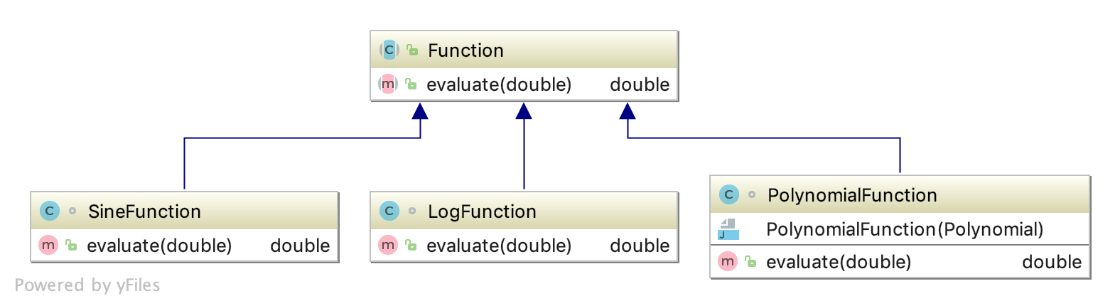

  

• A cleaner but more advanced way of representing functions is to use Java 8 lambda expressions and DoubleUnaryOperator. Replace Polynomial with DoubleUnaryOperator throughout AbstractRiemannExtended and its subclasses. This is an example of how those features could be used:

  // f(x) = sin(x) + cos(x) / 2
  DoubleUnaryOperator f = (x) -> Math.sin(x) + Math.cos(x) / 2;
  
  // Print f(4.9)
  System.out.println(f.applyAsDouble(4.9));
  
  // g(x) = poly.evaluateToNumber(x)
  DoubleUnaryOperator g = (x) -> poly.evaluateToNumber(x);
  
  // Print g(-2)
  System.out.println(g.applyAsDouble(-2));
  

Further Resources

Java/Computer Science

• Oracle - Inheritance
• Oracle - Abstract Classes and Methods
• Oracle - Interfaces
• freeCodeCamp.org - Lambda Expressions
• Math JavaDoc for the Math class - contains useful mathematical functions such as Math.sin() and Math.sqrt().

Math

• Wolfram Alpha - Can be used to calculate exact values of Riemann sums including arc lengths.