Getting Started

Welcome to CSX

CSX, also know as Advanced Math and Physics Modeling, is three classes taught in a unified manner. The classes are Precalculus 2A, Physics A, and Computer Science X. In teaching Math and Physics in a unified way, we recognize the historical development of the two subjects. Math and Physics fit together like a hand in a glove. It’s most instructive, and most enjoyable, if the two subjects are presented in tandem. In teaching Math, Physics, and Computer Science in a unified way, we recognize the way in which contemporary scientists work. Whereas once all scientists were either experimentalists or theorists – and most were experimentalists – scientists are now increasingly engaged in the creation of computer models. This has become a third way in which to understand the physical world. Computer models are based upon an understanding of the relevant Math and Science. However, through the use of a computer, relatively simple Math and Science can be used to model extremely complicated situations. Consequently, computer models are ubiquitous in areas as disparate as Global Warming and the Human Genome.

Almost all Computer Science projects will be based on Physics or Mathematics. Some programs will be computer models of physical situations. For example, you’ll model balls dropping, planets orbiting the Sun, and masses connected to a spring. Some programs will be realizations of mathematical algorithms. For instance, early on in the year you’ll write code to invert a matrix.

When possible, the same topics will be covered at the same time in both Math and Physics. Many of the concepts covered in Precalculus and Physics were developed simultaneously. Math is necessary for a deep understanding of Physics, and Physics provides beautiful applications of what would otherwise be abstract Mathematics.

We certainly hope you enjoy Math, Physics and Computer Science this year. In particular, we hope you find it helpful to approach the three subjects as, in some sense, one. Throughout the class, you should try to think about the ways in which Math is used in Physics, the ways in which Physics allows for a deeper understanding of Mathematics, and the ways in which computers could be used to gain a deeper understanding of either Math or Physics. In addition, bear in mind that Math and Physics provide a limitless source of programming challenges. Consequently, Math and Physics provide an excellent context in which to teach programming concepts.

Have a great year!

Setup your Environment

Follow these images to set up your environment:

Step 1. Open IntelliJ and select Get from VCS (top right button).

Step 2. In the URL box enter https://github.com/kjergens/XClassProjects.git and select Clone.

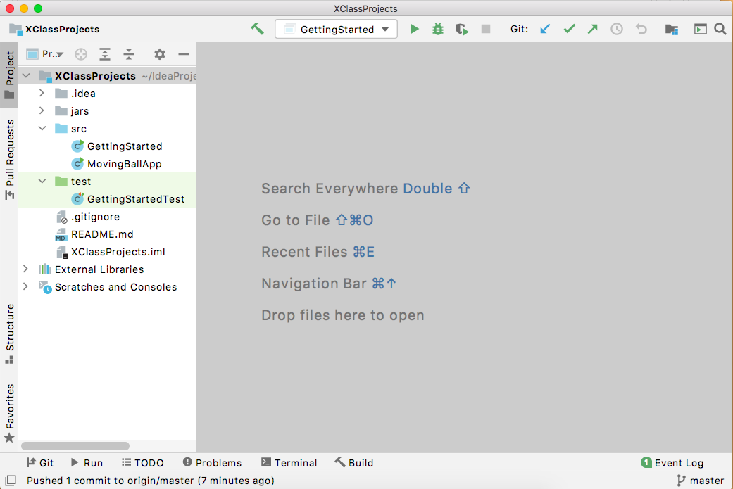
Step 3. Expand the src and test folders. These folders have example classes and are where you will put all your code for this course. Your project should look like the above.

Introduction to JUnit

For this section, you will review Quadratic equations, how to write objects and get introduced to writing test cases.

Problem: Find the roots of a Quadratic.

The x values that make this function equal to 0 are the roots or zeroes of the function and can be found by using the quadratic formula.

You are going to write a program that finds to roots (if they exist) for any quadratic equation.

Step 1: Create a Test Class

Exercise

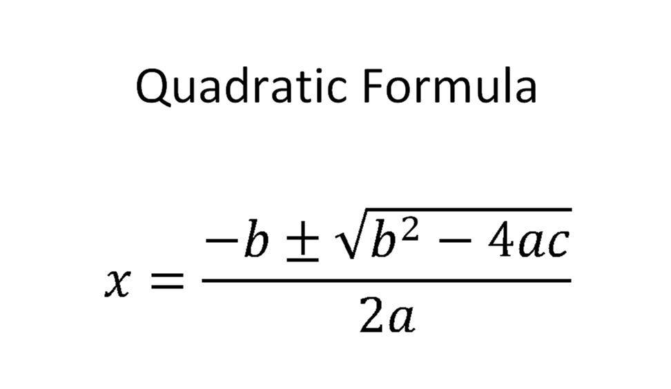
In the test folder of XClassProjects, create a new Java class called QuadraticTest. At the top of the class, import all the necessary JUnit libraries, like this:

import org.junit.Test;

import static org.hamcrest.core.Is.is;
import static org.junit.Assert.*;

In the body of the QuadraticTest class, create a test method called getA, like this:

@Test
public void getA() {
   Quadratic q = new Quadratic(1.0, 2.0, 3.0);

   assertThat(q.getA(), is(1.0));
}

If you need help, look at the GettingStartedTest class, in the test folder as an example.

Run the QuadraticTest class. It will fail at first, which is expected.

Step 2: Create a Quadratic Object

In order to get your test to pass, continue with the following exercise:

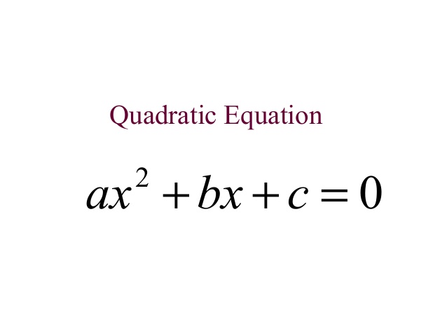
Exercise

1. In the src folder, create a new Java class called Quadratic. This will be the object class that defines a quadratic function and methods that analyze its different characteristics.

2. Create 3 private attributes a, b and c, all doubles.

3. Write a constructor which takes a, b and c as params and uses them to set the a, b and c attributes.

4. Write a public method called getA which returns the value of a.

5. Run QuadraticTest again. It should pass this time.

Step 3: Add Methods and Test methods

Once your QuadraticTest passes, continue with the following exercise:

Exercise

Note: For this exercise, you will switch back and forth between the Quadratic and QuadraticTest classes.

Write the following methods in Quadratic. For each method, write at least one test method in QuadraticTest.

1. public double getB()

   Return the value of b. In QuadraticTest and add test method for getB.

2. public double getC()

   Return the value of c. In QuadraticTest and add test method for getC.

3. public boolean hasRealRoots()

   See if the quadratic has real roots, return boolean true or false. Write a test method in QuadraticTest called hasRealRoots to test it .

4. public int numberOfRoots()

   Determine the number of real roots, return an int (0, 1, or 2). Write a test method in QuadraticTest called numberOfRoots to test it .

5. public double[] getRootArray()

   Find the roots, return 2 doubles (put them in an array). Write a test method in QuadraticTest called getRootArray to test it .

6. public double getAxisOfSymmetry()

   Find the axis of symmetry. Return that value. Write a test method in QuadraticTest called getAxisOfSymmetry to test it .

7. public double getExtremeValue()

   Find the extreme value, the maximum or minimum function value corresponding to the y coordinate of the vertex of the parabola. Return that value. Write a test method in QuadraticTest called getExtremeValue to test it .

8. public boolean isMax()

   Is the extreme value a Max or a Min? Does the parabola open up or down? Return true for Max and false for Min. Write a test method in QuadraticTest called isMax to test it .

9. public double evaluateWith(double x)

   Evaluate the quadratic function at an x value, return f(that x value). Write a test method in QuadraticTest called evaluateWith to test it .

When all the tests in QuadraticTest pass, you are finished with this exercise.

Introduction to Polyfun

Getting Started with Polynomials

Open the GettingStarted class and look at the Polynomial examples. (Ignore the rest of the code in the GettingStarted class for now.) Run the code and look at the output in the console. (Again, ignore the pop-up that appears for now.)

After looking over the code and the output, complete the following exercise.

Exercise

Do the following in the GettingStarted class.

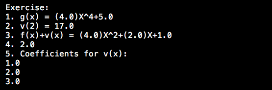
1. Create a Polynomial called gx and set it equal to (4.0)X^4 + 5.0. Print the Polynomial.

2. Evaluate vx for when x is 2 and print the answer.

3. Add fx and vx and print the answer.

4. For vx, print the coefficient for the X^1 term (also known as simply X).

5. Use a for-loop or for-each-loop to print all the coefficients of vx

When you get the output below you are finished with this exercise:

More Information

For more information, see the Polynomial JavaDocs.

Introduction to Open Source Physics (OSP)

Step 1: Plotting Polynomials (Static Graph)

Run the GettingStarted class again but this time look at the graph that appears. Hover over the graph for it to render. Look at the code under Open Source Physics (OSP) Example to see how this graph was made.

When you think you understand, do the following exercise:

Exercise

Do the following in the GettingStarted class.

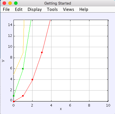
1. Look at the code that makes the red line. Comment out the lines that append points to the red line. Then use a for-loop to make the red line a graph of fx for when x is values 0 - 10.

2. Look at the code that makes the green line. Comment out the lines that append points to the green line. Then use a for-loop to make the green line a graph vx for when x is values 0 - 10.

3. Look at the code that makes the orange trail. Notice how this is different from the previous lines. Comment out the code that adds points to the trail. Then use a for-loop to make the orange line a graph of gx (which you created in the Introduction to Polyfun exercise) for when x is values 0 - 10.

When you get the output below you are finished with this exercise:

Which do you prefer, appending x and y plot points, or creating a Trail?

Step 2: Introduction to Animation

Open and run the MovingBallApp.

This is an example of an animation. It is different from a static graph, which you did in Step 1, in that you have to write at least three methods (reset, intialize, and doStep) in order for it to work.

Background Information: Abstract Classes

MovingBallApp is an extension of AbstractSimulation, an abstract class.

An abstract class is a class that is meant to be extended and one where the author left some methods empty, which are meant to be overridden. These empty methods are called abstract methods.

In AbstractSimulation, these are the abstract methods that MovingBallApp needs to override:

1. reset - Adds options to the Control Panel and returns the simulation to its default state. All commands within the reset() method are executed the FIRST time the simulation is INITIALIZED, and every time the RESET button is clicked after that. Note that the RESET button appears when the app is first loaded, but does not appear again until the app has been STARTED and STOPPED, and NEW is clicked.

2. initialize - Sets the initial conditions of your simulation. It should read and store values from the control panel and add objects to the PlotFrame. The commands within this method are executed once, or every time the INITIALIZE button in clicked.

3. doStep - Invoked every 1/10 second, it defines the actions that do the animation. It is also invoked each time the Step button is pressed.

You also need a main method to run the simulation.

Examine the MovingBallApp code, then do the following exercise.

Exercise

Do the following in the MovingBallApp class.

1. Add code to let the user set the starting X position of the ball.

2. Make the ball move diagonally across the graph, so as y decreases by 1, x simultaneously increases by 1.

When you get the output below you are finished with this exercise:

Step 3: Create Your Own Animation (Random Walk)

Now you’ll create an animation from scratch.

Exercise

1. In the src folder, create a new Java class called RandomWalkApp.

2. Copy and paste the MovingBallApp class as starter code. Change the main method to run RandomWalkApp.

3. Change doStep so that circle randomly moves plus or minus 0.5 pixels vertically and plus or minus 0.5 pixels horizontally.

   

4. Add 50 Circles that move in this way.

When you get output similar to the graph below you are finished with this exercise:

HINT: Change the global circle variable to an array of type Circle called circles.

HINT: Use a for-loop in initialize to add 50 Circles to circles, and another one in do-step to move each Circle in circles.

Step 4: (Advanced) Spiral Trail Animation

Exercise

For this exercise, you have to determine on your own to which method - reset, initialize, or doStep - to edit for each step.

Note: If you like, you may first make this a static graph, and then change it to an animation.

1. In src folder, Create a new Java class called SpiralTrailApp. The class should extend AbstractSimulation.

2. Set up empty methods for reset, initialize, and doStep.

3. Add a main method to run the simulation.

4. Create a rectangle using the DrawableShape.createRectangle() method like this:

// The x and y parameters place the center of the rectangle.
DrawableShape rect = DrawableShape.createRectangle(x, y, width, height);

5. Edit the rectangle to be a square with the lower left corner at (1,1) and upper right corner at (5,5). Note that the x and y represent the center of the rectangle, not the upper left corner.

6. Create a PlotFrame and add the square.

7. Set the PlotFrame’s preferred min and max x and y so that the square is in the middle of the plot frame.

8. On the PlotFrame draw a circle centered at each of the lattice points contained in the square. (There should be a total of 25 circles.)

9. Draw a Trail that starts at the origin, (3, 3), and “steps” outward in a spiral-like shape by first going to (2, 3), then (2, 2), (4, 2), etc. The path should consist of 2 segments of length 1, then 2 segments of length 2, then 2 segments of length 3, etc. and the path turns 90° counter clockwise at the end of each segment. End the Trail at (1, 5).

When you get the output below you are finished with this exercise:

More Information

For more information on Open Source Physics, read the Open Source Physics JavaDocs